Results
Figure 1 shows the distribution of fall prices for both 100% harvest sale (no hedging) and a hedging strategy where the initial price is $6.10 per bushel. The hedging strategy involves hedging 40% of expected production using the “Terry Timer” approach of 10 equally sized sales spaced 10 days apart starting on March 1 and 60% of expected production sold on November 1. Figure 1 shows that hedging using a 40% portfolio improves marketing outcomes by reducing the probability of receiving low prices, point A, at the expense of reducing the probability of receiving very high prices, point B. Hedging creates a portfolio of prices causing your average price to move lower or higher at a slower speed than doing nothing. When prices drop, your average price drops, but not to the point of doing nothing. This result is why hedging reduces risk. When prices increase, your average price increases, but not to the point of doing nothing. The point here is to view hedging as a portfolio of prices, allowing you to create an average farm price. Hedging seems to hurt more when prices go up in the fall, however, when you view your hedge as a portfolio, your farm average price increases as your unsold bushels are worth more.
Figure 1, Average Farm Fall Price Distribution with and without Hedging
In our latest article
we identified that December corn futures prices have, on average, historically tended to drift lower from spring to fall. This drift is commonly known as the seasonal price signal. Many market advisors use this observation to encourage producers to price some of their expected production in the spring or early summer. Selling pre-harvest comes with risk. The seasonal is based on the average over many years of data. However, each producer’s marketing performance is measured each year. Each year matters because a farmer’s financial performance is measured at the end of every year. Selling in the spring implies the producer accepts what the market is offering instead of waiting for potentially higher prices later in the year. However, no one wants to be wrong! A marketing plan based on the seasonal could show excellent long-term returns but lose a substantial amount of money in any given year. The effect on yearly price risk needs to be considered.
In 2022 corn prices started high and ended higher while during the growing season, moved higher and lower than the spring price. The corn time price path for 2022 is shown in Figure 2.
Figure 2, 2022 December Corn Price as a function of Marketing Days
Marketing is especially important in a period of high prices and high volatility such as 2022. Corn futures started at $6.24 on March 1, peaked at $7.66 on May 16, bottomed at $5.64 on Jul 22, and ended at $6.97 on Nov 1. Producers had the opportunity to price any part of their production on each marketing day between March 1 and November 1. The difference in pricing production on May 16 versus July 22 is about $388.00 per acre (($7.66-$5.64) *193 bushels per acre) for a typical Colfax County NE producer who produces corn under rain-fed conditions. With high input prices, $388 makes a difference in a farm’s bottom line and could be the difference between a profit and loss.
From the above discussion, hedging is both difficult and financially important. We now turn to hedging 2023 corn crop where the price/cost squeeze is taking place as production costs are higher than in 2022 and December 2023 futures prices trading around $6.10 per bushel, a similar price found on March 1, 2022.
Time-Dependent Model
We first lay out the framework in which decisions will be made. First, fall prices will be revealed when we get to the fall, and we cannot predict fall price beforehand. Second, the hedging decision happens before the fall price is known, so we must make the decision looking into an unknown future. Third, the path in which prices evolve from the spring to the fall will be unique. There are thousands of possible price paths, yet we see only one each year. It is here, the path prices take that matters so much. We only observe one price path per year, but there exist thousands of possibilities. Fourth, probability of 2023 corn futures price path being like 2022 is close to zero.
What do we do? We model price evolution of thousands of potential paths by allowing prices to evolve through random shocks. Shocks that could reflect wars, production issues, etc.… We then include hedging into this model and observe the changes in price outcomes. Here, price outcomes are defined as the average farm price since the farm sells some crop through the hedge and the rest at harvest.
The time period we are considering here is from March 1 to November 1, the pre-harvest time frame. For simplicity, we are focusing on daily moves. Each day the farmer can sell at the closing price or wait until the next day for new closing price. For example, on March 1, the market absorbs the available supply and demand information and establishes a consensus price that represents an equilibrium between potential buyers and sellers. On March 1 the farmer has the choice to sell some, or all, of her anticipated production at the price the market offers or wait until the next day. As new information arrives, the market adjusts. The farmer can accept the new market consensus by pricing part of her crop or wait for a possibly better offer the next day. This leads to a daily recurrent process continuing until the history of sales along a particular time-dependent path is tallied at a preset ending point, November 1 in this analysis. Sales occur along a possible path. With this, we assume that Ln prices meander through time following a Generalized Browning Motion Stochastic Model,
(1) ? [Ln(P)] = (μ – σ^2/2) ?t +σ ε(?t)^(1/2)
where ε represents the standard normal distribution, μ represents the drift, σ represents the implied volatility. This process represents a simple explanation of the marketing mystery. Each day the price changes by the deterministic first term and a random part that represents new information arriving in the marketplace. Monte Carlo estimates the results implied by equation 1 by sampling this equation with many different paths. Each path experiences a different random exposure to information each day. Historical seasonality (i.e., piecewise drift) is added to the model framework and the resulting differential equation is solved numerically. Today's computers and the availability of modern software applications, such as Analytica, make it possible to conduct this intensive numerical calculation. This improved technology lets the producer do the thinking while the computer does the work.
The “Terry Timer” Marketing Plan
When tested using historical yearly data, Zimmerman et. al. 2021found that a marketing plan based on selling a certain amount of production at fixed times throughout the year outperformed sell nothing until harvest plan as well as multiple other marketing plans. Ed Usset clearly discusses how different marketing plans have performed in his introduction to marketing, Grain Marketing is Simple (It’s Just Not Easy). We incorporate this marketing plan into our stochastic model. For Terry Timer, we make 10 equally sized sales 10 days apart on each path, figure 3. The last sale is completed in early July. This approach makes sure that the sales are clustered in the spring to exploit the seasonal tendency for prices to be higher in the spring than the final fall price. We produce a probability distribution of possible outcomes rather than a simple point estimate of the future. By assuming that our 30,000 paths can be thought of as 30,000 years, the average or expectation of this distribution gives us an estimate of the long-run performance of the “Terry Timer” model.

Figure 3, Ten Terry Timer Marketing Points
Hedging Alone
To simplify the complexities of farm management decision making Agricultural Economists often present hedging as a separate enterprise. Once it is separated it is assumed that hedging is recommended if it produces a profit. In this reductionist view, hedging value is measured as the difference of selling expected production using a marketing plan or not, given by
(1) Hedge Valuen = Market Plann- Fall Pricen
for each possible path n. Often, for simplicity, only the average is reported. Using our modified drift adaption, the average value for using “Terry Timer” hedging plan is projected to be $0.34. The results for 30,000 paths using the “Terry Timer” plan are shown in figure 4.
Figure 4, Hedge Value, Equation2
It has been common practice to only compare the average. The average is a positive $34 when using the “Terry Timer” marketing plan. However, this view, where we show yearly outcomes, clearly identifies that a producer can lose money in his hedge account in any given year. Some years it can be a lot of money – the negative values. In those years the producer is going to have to explain to his spouse or banker why he hedged at all. This view presents the reductionist view of hedging, that hedging can be treated as a separate entity.
Hedging Your Price Portfolio
Hedging is not a separate entity and success cannot be judged alone. It is better to view hedging in a portfolio where you include the price on unhedged production. Figure 5 shows the distribution of possible price outcomes of a hedging portfolio that includes 40% of expected production sold using the “Terry Timer” model and 60% unsold starting on March 1 for both the November 1 fall price and the price outcome using the “Terry Timer” model hedging 40% of projected production. (On Mar 1 only the distribution of possible prices can be forecast.)
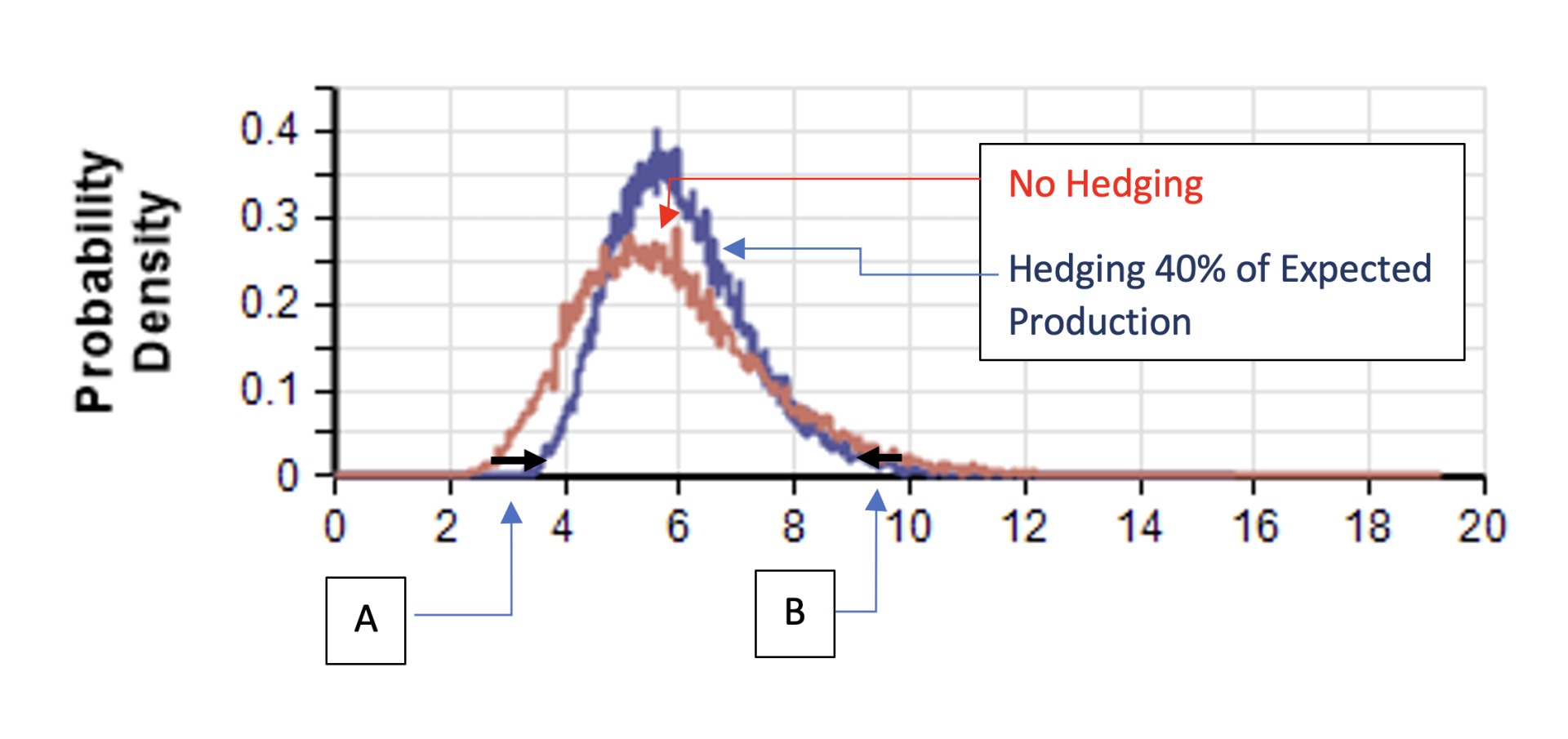
Figure 5, Average Farm Price Distribution with and without Hedging
Figure 5 shows that hedging using a 40% portfolio improves marketing outcomes by reducing the probability of receiving low prices (point A) at the expense of reducing the probability of receiving very high prices (point B). The “Terry Timer” model exploits the seasonal tendency for prices to drift lower from spring to fall. Therefore, the Terry Timer marketing plan obtains an improved result when many paths are averaged together. The width of the no hedging distribution gives the uncertainty that a producer is faced with in the spring. Hedging 40% of expected production reduces uncertainty. If risk is defined as obtaining a low price, then hedging 40% reduces risk. However, if risk is defined as not obtaining the highest price in the community each year, then hedging increases this type of risk. Risk is personal as risk depends on each individual’s perception of the future and goals.
Summary
Hedging influences your farm average price. We encourage you to focus on this viewpoint. Not that we are encouraging you to engage in hedging, as this is a personal decision, rather, that when you are deciding whether to hedge, base the decision on creating a farm average price.
While our focus was on hedging, production risk also exists. While a hedge sets a price, which reduces uncertainty, it increases production risk. If production falls short of the amount hedged and the fall price turns out higher than the average hedge price, these shortfall bushels must be bought back at the higher price. This is an added risk introduced by hedging, an unintended consequence. Limiting hedging to a percent of expected production and purchasing a revenue-based crop insurance policy at a reasonable coverage level provides financial protection from buying back contracts. Future articles will examine the complete risk profile faced by individual farms and discuss how hedging, crop insurance, and working capital interact to improve outcomes and reduce risk.
Source : unl.edu